Future: Parallel & Distributed Processing in R for Everyone

Animation: Formula 1 pitstop parallel team work

Henrik Bengtsson

University of California

@HenrikBengtsson

HenrikBengtsson/future

jottr.org

Acknowledgments
- eRum 2018
- R Consortium
- R Core, CRAN, devels & users!

A 20-minute presentation, eRum 2018, Budapest, 2018-05-16

Why do we parallelize software?

Parallel & distributed processing can be used to:

speed up processing (wall time)
decrease memory footprint (per machine)
avoid data transfers

Comment: I'll focuses on the first two in this talk.

2 / 23

Definition: Future

A future is an abstraction for a value that will be available later
The value is the result of an evaluated expression
The state of a future is unevaluated or evaluated

Friedman & Wise (1976, 1977), Hibbard (1976), Baker & Hewitt (1977)

3 / 23

Definition: FutureA future is an abstraction for a value that will be available later
The value is the result of an evaluated expression
The state of a future is unevaluated or evaluated

Standard R:
v <- expr

3 / 23

Definition: FutureA future is an abstraction for a value that will be available later
The value is the result of an evaluated expression
The state of a future is unevaluated or evaluated

Standard R:
v <- expr


Future API:
f <- future(expr)
v <- value(f)

3 / 23

Example: Sum of 1:50 and 51:100 in parallel

> library(future)
> plan(multiprocess)

4 / 23

Example: Sum of 1:50 and 51:100 in parallel

> library(future)
> plan(multiprocess)
> fa <- future( slow_sum( 1:50 ) )
>

4 / 23

Example: Sum of 1:50 and 51:100 in parallel

> library(future)
> plan(multiprocess)
> fa <- future( slow_sum( 1:50 ) )
> fb <- future( slow_sum(51:100) )
>

4 / 23

Example: Sum of 1:50 and 51:100 in parallel

> library(future)
> plan(multiprocess)
> fa <- future( slow_sum( 1:50 ) )
> fb <- future( slow_sum(51:100) )
> 1:3
[1] 1 2 3
>

4 / 23

Example: Sum of 1:50 and 51:100 in parallel

> library(future)
> plan(multiprocess)
> fa <- future( slow_sum( 1:50 ) )
> fb <- future( slow_sum(51:100) )
> 1:3
[1] 1 2 3
> value(fa)

4 / 23

Example: Sum of 1:50 and 51:100 in parallel

> library(future)
> plan(multiprocess)
> fa <- future( slow_sum( 1:50 ) )
> fb <- future( slow_sum(51:100) )
> 1:3
[1] 1 2 3
> value(fa)
[1] 1275

4 / 23

Example: Sum of 1:50 and 51:100 in parallel

> library(future)
> plan(multiprocess)
> fa <- future( slow_sum( 1:50 ) )
> fb <- future( slow_sum(51:100) )
> 1:3
[1] 1 2 3
> value(fa)
[1] 1275
> value(fb)
[1] 3775

4 / 23

Example: Sum of 1:50 and 51:100 in parallel

> library(future)
> plan(multiprocess)
> fa <- future( slow_sum( 1:50 ) )
> fb <- future( slow_sum(51:100) )
> 1:3
[1] 1 2 3
> value(fa)
[1] 1275
> value(fb)
[1] 3775
> value(fa) + value(fb)
[1] 5050

4 / 23

Definition: Future
Standard R:
v <- expr


Future API (implicit):
v %<-% expr

5 / 23

Example: Sum of 1:50 and 51:100 in parallel (implicit API)

> library(future)
> plan(multiprocess)
> a %<-% slow_sum( 1:50 )
> b %<-% slow_sum(51:100)
> 1:3
[1] 1 2 3
> a + b
[1] 5050

6 / 23

Many ways to resolve futures

plan(sequential)
plan(multiprocess)
plan(cluster, workers = c("n1", "n2", "n3"))
plan(cluster, workers = c("remote1.org", "remote2.org"))
...

7 / 23

Many ways to resolve futures

plan(sequential)
plan(multiprocess)
plan(cluster, workers = c("n1", "n2", "n3"))
plan(cluster, workers = c("remote1.org", "remote2.org"))
...

> a %<-% slow_sum( 1:50 )
> b %<-% slow_sum(51:100)
> a + b
[1] 5050

7 / 23

R package: future

"Write once, run anywhere"
A simple unified API ("interface of interfaces")
100% cross platform
Easy to install (~0.4 MiB total)
Very well tested, lots of CPU mileage, production ready

╔════════════════════════════════════════════════════════╗
║                     < Future API >                     ║
║                                                        ║
║              future(), value(), %<-%, ...              ║
╠════════════════════════════════════════════════════════╣
║                         future                         ║
╠════════════════════════════════╦═══════════╦═══════════╣
║            parallel            ║  globals  ║ (listenv) ║
╠══════════╦══════════╦══════════╬═══════════╬═══════════╝
║   snow   ║   Rmpi   ║   nws    ║ codetools ║
╚══════════╩══════════╩══════════╩═══════════╝

8 / 23

Why a Future API? Problem: heterogeneity

Different parallel backends ⇔ different APIs
Choosing API/backend, limits user's options

x <- list(a = 1:50, b = 51:100)
y <- lapply(x, FUN = slow_sum)

9 / 23

Why a Future API? Problem: heterogeneity

Different parallel backends ⇔ different APIs
Choosing API/backend, limits user's options

x <- list(a = 1:50, b = 51:100)
y <- lapply(x, FUN = slow_sum)

y <- parallel::mclapply(x, FUN = slow_sum)

9 / 23

Why a Future API? Problem: heterogeneity

Different parallel backends ⇔ different APIs
Choosing API/backend, limits user's options

x <- list(a = 1:50, b = 51:100)
y <- lapply(x, FUN = slow_sum)

y <- parallel::mclapply(x, FUN = slow_sum)

library(parallel)
cluster <- makeCluster(4)
y <- parLapply(cluster, x, fun = slow_sum)
stopCluster(cluster)

9 / 23

Why a Future API? Solution: "interface of interfaces"

The Future API encapsulates heterogeneity
- fever decisions for developer to make
- more power to the end user
Philosophy:
- developer decides what to parallelize - user decides how to
Provides atomic building blocks for richer parallel constructs, e.g. 'foreach' and 'future.apply'
Easy to implement new backends, e.g. 'future.batchtools' and 'future.callr'

10 / 23

Why a Future API? 99% Worry Free

Globals: automatically identified & exported
Packages: automatically identified & exported
Static-code inspection by walking the AST

x <- rnorm(n = 100)
y <- future({ slow_sum(x) })

Why a Future API? 99% Worry Free

Globals: automatically identified & exported
Packages: automatically identified & exported
Static-code inspection by walking the AST

x <- rnorm(n = 100)
y <- future({ slow_sum(x) })

Globals identified and exported:

slow_sum() - a function (also searched recursively)

Why a Future API? 99% Worry Free

Globals: automatically identified & exported
Packages: automatically identified & exported
Static-code inspection by walking the AST

x <- rnorm(n = 100)
y <- future({ slow_sum(x) })

Globals identified and exported:

slow_sum() - a function (also searched recursively)
x - a numeric vector of length 100

Why a Future API? 99% Worry Free

Globals: automatically identified & exported
Packages: automatically identified & exported
Static-code inspection by walking the AST

x <- rnorm(n = 100)
y <- future({ slow_sum(x) })

Globals identified and exported:

slow_sum() - a function (also searched recursively)
x - a numeric vector of length 100

Globals & packages can be specified manually too

High Performance Compute (HPC) clusters

Future Art: Mainframe computer room

Backend: future.batchtools

batchtools: Map-Reduce API for HPC schedulers,
e.g. LSF, OpenLava, SGE, Slurm, and TORQUE / PBS
future.batchtools: Future API on top of batchtools

╔═══════════════════════════════════════════════════╗
║                   < Future API >                  ║
╠═══════════════════════════════════════════════════╣
║          future        <->   future.batchtools    ║
╠═════════════════════════╦═════════════════════════╣
║         parallel        ║        batchtools       ║
╚═════════════════════════╬═════════════════════════╣
                          ║ SGE, Slurm, TORQUE, ... ║
                          ╚═════════════════════════╝

12 / 23

Backend: future.batchtools

> library(future.batchtools)
> plan(batchtools_sge)
> a %<-% slow_sum(1:50)
> b %<-% slow_sum(51:100)
> a + b
[1] 5050

13 / 23

Real Example: DNA Sequence Analysis

DNA sequences from 100 cancer patients
200 GiB data / patient (~ 10 hours)

raw <- dir(pattern = "[.]fq$")
aligned <- listenv()
for (i in seq_along(raw)) {
  aligned[[i]] %<-% DNAseq::align(raw[i])
}
aligned <- as.list(aligned)

Real Example: DNA Sequence Analysis

DNA sequences from 100 cancer patients
200 GiB data / patient (~ 10 hours)

raw <- dir(pattern = "[.]fq$")
aligned <- listenv()
for (i in seq_along(raw)) {
  aligned[[i]] %<-% DNAseq::align(raw[i])
}
aligned <- as.list(aligned)

plan(multiprocess)
plan(cluster, workers = c("n1", "n2", "n3"))
plan(batchtools_sge)

Comment: The use of `listenv` is non-critical and only needed for implicit futures when assigning them by index (instead of by name).

Building on top of Future API

Funny car

Frontend: future.apply

Futurized version of base R's lapply(), vapply(), replicate(), ...
... on all future-compatible backends

╔═══════════════════════════════════════════════════════════╗
║ future_lapply(), future_vapply(), future_replicate(), ... ║
╠═══════════════════════════════════════════════════════════╣
║                       < Future API >                      ║
╠═══════════════════════════════════════════════════════════╣
║                         "wherever"                        ║
╚═══════════════════════════════════════════════════════════╝

aligned <- lapply(raw, DNAseq::align)

15 / 23

Frontend: future.apply

Futurized version of base R's lapply(), vapply(), replicate(), ...
... on all future-compatible backends

╔═══════════════════════════════════════════════════════════╗
║ future_lapply(), future_vapply(), future_replicate(), ... ║
╠═══════════════════════════════════════════════════════════╣
║                       < Future API >                      ║
╠═══════════════════════════════════════════════════════════╣
║                         "wherever"                        ║
╚═══════════════════════════════════════════════════════════╝

aligned <- future_lapply(raw, DNAseq::align)

16 / 23

Frontend: future.apply

Futurized version of base R's lapply(), vapply(), replicate(), ...
... on all future-compatible backends

╔═══════════════════════════════════════════════════════════╗
║ future_lapply(), future_vapply(), future_replicate(), ... ║
╠═══════════════════════════════════════════════════════════╣
║                       < Future API >                      ║
╠═══════════════════════════════════════════════════════════╣
║                         "wherever"                        ║
╚═══════════════════════════════════════════════════════════╝

aligned <- future_lapply(raw, DNAseq::align)

plan(multiprocess)
plan(cluster, workers = c("n1", "n2", "n3"))
plan(batchtools_sge)

16 / 23

Frontend: doFuture

A foreach adapter on top of the Future API
Foreach on all future-compatible backends

╔═══════════════════════════════════════════════════════╗
║                      foreach API                      ║
╠════════════╦══════╦════════╦═══════╦══════════════════╣
║ doParallel ║ doMC ║ doSNOW ║ doMPI ║     doFuture     ║
╠════════════╩══╦═══╩════════╬═══════╬══════════════════╣
║   parallel    ║    snow    ║ Rmpi  ║  < Future API >  ║
╚═══════════════╩════════════╩═══════╬══════════════════╣
                                     ║    "wherever"    ║
                                     ╚══════════════════╝

doFuture::registerDoFuture()
plan(batchtools_sge)
aligned <- foreach(x = raw) %dopar% {
  DNAseq::align(x)
}

17 / 23

1,200+ packages can now parallelize on HPC

┌───────────────────────────────────────────────────────┐
│                                                       │
│      caret, gam, glmnet, plyr, ... (1,200 pkgs)       │
│                                                       │
╠═══════════════════════════════════════════════════════╣
║                      foreach API                      ║
╠══════╦════════════╦════════╦═══════╦══════════════════╣
║ doMC ║ doParallel ║ doSNOW ║ doMPI ║     doFuture     ║
╠══════╩════════╦═══╩════════╬═══════╬══════════════════╣
║   parallel    ║    snow    ║ Rmpi  ║  < Future API >  ║
╚═══════════════╩════════════╩═══════╬══════════════════╣
                                     ║    "wherever"    ║
                                     ╚══════════════════╝

doFuture::registerDoFuture()
plan(future.batchtools::batchtools_sge)
library(caret)
model <- train(y ~ ., data = training)

## 2018-05-12
> db <- utils::available.packages()
> direct <- tools::dependsOnPkgs("foreach", recursive=FALSE, installed=db)
> str(direct)
 chr [1:443] "adabag" "admixturegraph" "ADMMsigma" "Arothron" "ashr" ...
> all <- tools::dependsOnPkgs("foreach", recursive=TRUE, installed=db)
> str(all)
 chr [1:1200] "adabag" "admixturegraph" "ADMMsigma" "Arothron" "ashr" ...

Futures in the Wild

Frontend: drake - A Workflow Manager

tasks <- drake_plan(
  raw_data = readxl::read_xlsx(file_in("raw-data.xlsx")),
  data = raw_data %>% mutate(Species =
         forcats::fct_inorder(Species)) %>% select(-X__1),
  hist = ggplot(data, aes(x = Petal.Width, fill = Species))
         + geom_histogram(),
  fit = lm(Sepal.Width ~ Petal.Width + Species, data),
  rmarkdown::render(knitr_in("report.Rmd"),
                    output_file = file_out("report.pdf"))
)
future::plan("multiprocess")
make(tasks, parallelism = "future")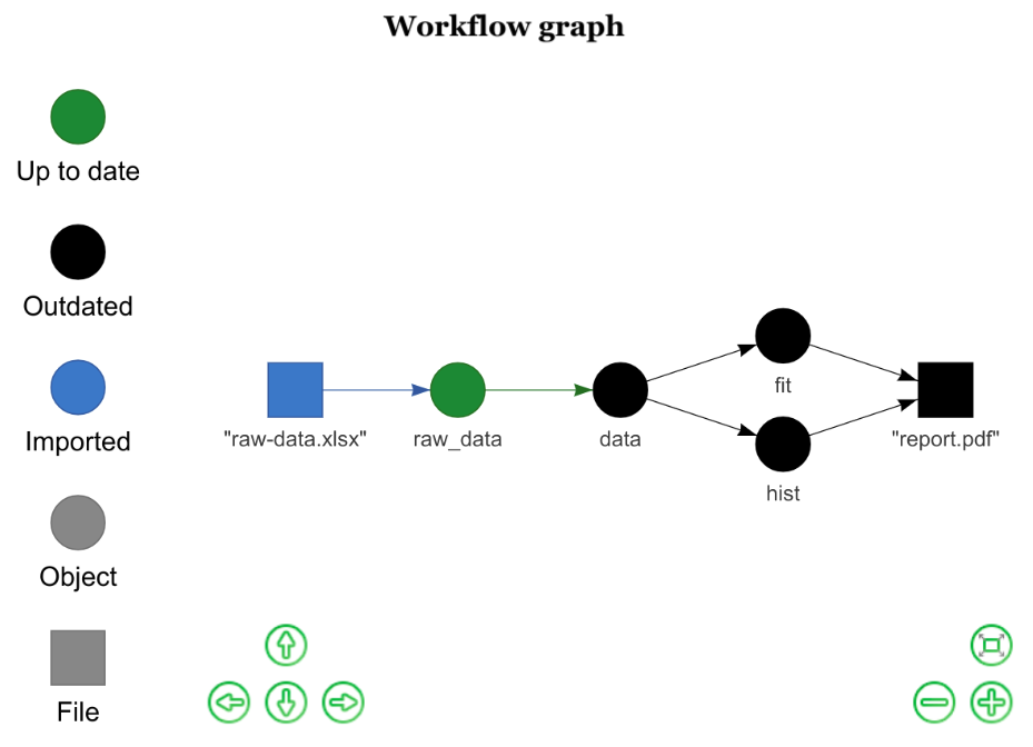

19 / 23

Screenshot of drake workflow graph

20 / 23

shiny - Now with Asynchronous UI

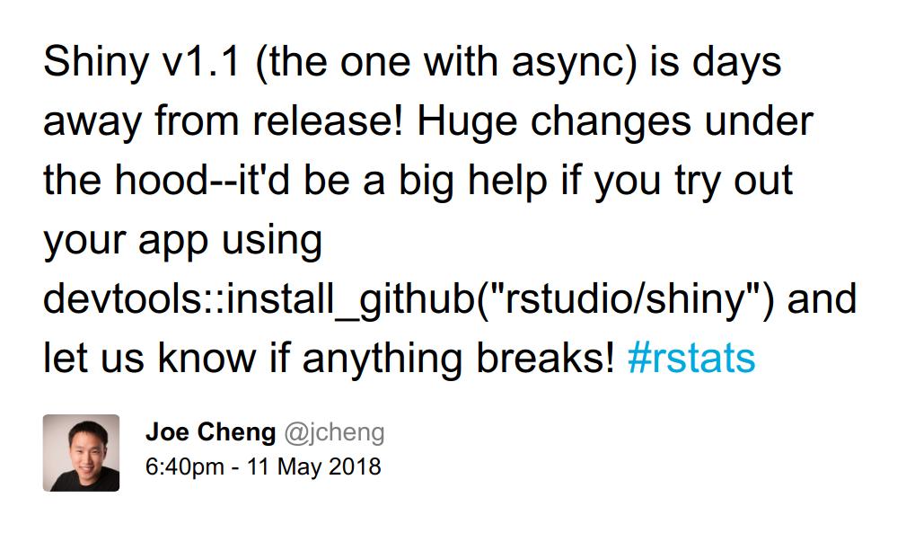
library(shiny)
future::plan("multiprocess")
...

21 / 23

Summary of features

Unified API
Portable code
Worry-free
Developer decides what to parallelize - user decides how to
For beginners as well as advanced users
Nested parallelism on nested heterogeneous backends
Protects against recursive parallelism
Easy to add new backends
Easy to build new frontends

22 / 23

In the near future ...Capturing standard output
Benchmarking (time and memory)
Killing futures

Building a better future

I 💜 feedback,
bug reports,
and suggestions

@HenrikBengtsson

HenrikBengtsson/future

jottr.org

Thank you!

Appendix (Random Slides)

A1. Features - more details

A1.1 Well Tested

Large number of unit tests
System tests
High code coverage (union of all platform near 100%)
Cross platform testing
CI testing
Testing several R versions (many generations back)
Reverse package dependency tests
All backends highly tested
Large of tests via doFuture across backends on example():s from foreach, NMF, TSP, glmnet, plyr, caret, etc. (example link)

R Consortium Infrastructure Steering Committee (ISC) Support Project

Backend Conformance Test Suite - an effort to formalizing and standardizing the above tests into a unified go-to test environment.

A1.2 Nested futures

raw <- dir(pattern = "[.]fq$")
aligned <- listenv()
for (i in seq_along(raw)) {
  aligned[[i]] %<-% {  
    chrs <- listenv()
    for (j in 1:24) {
      chrs[[j]] %<-% DNAseq::align(raw[i], chr = j)
    }
    merge_chromosomes(chrs)
  }
}

A1.2 Nested futures

raw <- dir(pattern = "[.]fq$")
aligned <- listenv()
for (i in seq_along(raw)) {
  aligned[[i]] %<-% {  
    chrs <- listenv()
    for (j in 1:24) {
      chrs[[j]] %<-% DNAseq::align(raw[i], chr = j)
    }
    merge_chromosomes(chrs)
  }
}

plan(batchtools_sge)

A1.2 Nested futures

raw <- dir(pattern = "[.]fq$")
aligned <- listenv()
for (i in seq_along(raw)) {
  aligned[[i]] %<-% {  
    chrs <- listenv()
    for (j in 1:24) {
      chrs[[j]] %<-% DNAseq::align(raw[i], chr = j)
    }
    merge_chromosomes(chrs)
  }
}

plan(batchtools_sge)
plan(list(batchtools_sge, sequential))

A1.2 Nested futures

raw <- dir(pattern = "[.]fq$")
aligned <- listenv()
for (i in seq_along(raw)) {
  aligned[[i]] %<-% {  
    chrs <- listenv()
    for (j in 1:24) {
      chrs[[j]] %<-% DNAseq::align(raw[i], chr = j)
    }
    merge_chromosomes(chrs)
  }
}

plan(batchtools_sge)
plan(list(batchtools_sge, sequential))
plan(list(batchtools_sge, multiprocess))

A1.3 Lazy evaluation

By default all futures are resolved using eager evaluation, but the developer has the option to use lazy evaluation.

Explicit API:

f <- future(..., lazy = TRUE)
v <- value(f)

Implicit API:

v %<-% { ... } %lazy% TRUE

A1.4 False-negative & false-positive globals

Identification of globals from static-code inspection has limitations (but defaults cover a large number of use cases):

False negatives, e.g. my_fcn is not found in do.call("my_fcn", x). Avoid by using do.call(my_fcn, x).
False positives - non-existing variables, e.g. NSE and variables in formulas. Ignore and leave it to run-time.

x <- "this FP will be exported"
data <- data.frame(x = rnorm(1000), y = rnorm(1000))
fit %<-% lm(x ~ y, data = data)

Comment: ... so, the above works.

A1.5 Full control of globals (explicit API)

Automatic (default):

x <- rnorm(n = 100)
y <- future({ slow_sum(x) }, globals = TRUE)

By names:

y <- future({ slow_sum(x) }, globals = c("slow_sum", "x"))

As name-value pairs:

y <- future({ slow_sum(x) }, globals =
                                 list(slow_sum = slow_sum, x = rnorm(n = 100)))

Disable:

y <- future({ slow_sum(x) }, globals = FALSE)

A1.5 Full control of globals (implicit API)

Automatic (default):

x <- rnorm(n = 100)
y %<-% { slow_sum(x) } %globals% TRUE

By names:

y %<-% { slow_sum(x) } %globals% c("slow_sum", "x")

As name-value pairs:

y %<-% { slow_sum(x) } %globals% list(slow_sum = slow_sum, x = rnorm(n = 100))

Disable:

y %<-% { slow_sum(x) } %globals% FALSE

A1.6 Protection: Exporting too large objects

x <- lapply(1:100, FUN = function(i) rnorm(1024 ^ 2))
y <- list()
for (i in seq_along(x)) {
  y[[i]] <- future( mean(x[[i]]) )
}

gives error: "The total size of the 2 globals that need to be exported for the future expression ('mean(x[[i]])') is 800.00 MiB. This exceeds the maximum allowed size of 500.00 MiB (option 'future.globals.maxSize'). There are two globals: 'x' (800.00 MiB of class 'list') and 'i' (48 bytes of class 'numeric')."

A1.6 Protection: Exporting too large objects

x <- lapply(1:100, FUN = function(i) rnorm(1024 ^ 2))
y <- list()
for (i in seq_along(x)) {
  y[[i]] <- future( mean(x[[i]]) )
}

for (i in seq_along(x)) {
  x_i <- x[[i]]  ## Fix: subset before creating future
  y[[i]] <- future( mean(x_i) )
}

Comment: Interesting research project to automate via code inspection.

A1.7 Free futures are resolved

Implicit futures are always resolved:

a %<-% sum(1:10)
b %<-% { 2 * a }
print(b)
## [1] 110

A1.7 Free futures are resolved

Implicit futures are always resolved:

a %<-% sum(1:10)
b %<-% { 2 * a }
print(b)
## [1] 110

Explicit futures require care by developer:

fa <- future( sum(1:10) )
a <- value(fa)
fb <- future( 2 * a )

A1.7 Free futures are resolved

Implicit futures are always resolved:

a %<-% sum(1:10)
b %<-% { 2 * a }
print(b)
## [1] 110

Explicit futures require care by developer:

fa <- future( sum(1:10) )
a <- value(fa)
fb <- future( 2 * a )

For the lazy developer - not recommended (may be expensive):

options(future.globals.resolve = TRUE)
fa <- future( sum(1:10) )
fb <- future( 2 * value(fa) )

A1.8 What's under the hood?

Future class and corresponding methods:
- abstract S3 class with common parts implemented,
  e.g. globals and protection
- new backends extend this class and implement core methods,
  e.g. value() and resolved()
- built-in classes implement backends on top the parallel package

A1.9 Universal union of parallel frameworks

	future	parallel	foreach	batchtools	BiocParallel
Synchronous	✓	✓	✓	✓	✓
Asynchronous	✓	✓	✓	✓	✓
Uniform API	✓		✓	✓	✓
Extendable API	✓		✓	✓	✓
Globals	✓		(✓)
Packages	✓
Map-reduce ("lapply")	✓	✓	`foreach()`	✓	✓
Load balancing	✓	✓	✓	✓	✓
For loops	✓
While loops	✓
Nested config	✓
Recursive protection	✓	mc	mc	mc	mc
RNG stream	✓+	✓	doRNG	(soon)	SNOW
Early stopping	✓				✓
Traceback	✓				✓

A2 Bells & whistles

A2.1 availableCores() & availableWorkers()

availableCores() is a "nicer" version of parallel::detectCores() that returns the number of cores allotted to the process by acknowledging known settings, e.g.
- getOption("mc.cores")
- HPC environment variables, e.g. NSLOTS, PBS_NUM_PPN, SLURM_CPUS_PER_TASK, ...
- _R_CHECK_LIMIT_CORES_

availableWorkers() returns a vector of hostnames based on:
- HPC environment information, e.g. PE_HOSTFILE, PBS_NODEFILE, ...
- Fallback to rep("localhost", availableCores())

Provide safe defaults to for instance

plan(multiprocess)
plan(cluster)

A2.2: makeClusterPSOCK()

makeClusterPSOCK():

Improves upon parallel::makePSOCKcluster()
Simplifies cluster setup, especially remote ones
Avoids common issues when workers connect back to master:
- uses SSH reverse tunneling
- no need for port-forwarding / firewall configuration
- no need for DNS lookup
Makes option -l <user> optional (such that ~/.ssh/config is respected)

A2.3 HPC resource parameters

With 'future.batchtools' one can also specify computational resources, e.g. cores per node and memory needs.

plan(batchtools_sge, resources = list(mem = "128gb"))
y %<-% { large_memory_method(x) }

Specific to scheduler: resources is passed to the job-script template where the parameters are interpreted and passed to the scheduler.

A2.3 HPC resource parameters

With 'future.batchtools' one can also specify computational resources, e.g. cores per node and memory needs.

plan(batchtools_sge, resources = list(mem = "128gb"))
y %<-% { large_memory_method(x) }

Specific to scheduler: resources is passed to the job-script template where the parameters are interpreted and passed to the scheduler.

Each future needs one node with 24 cores and 128 GiB of RAM:

resources = list(l = "nodes=1:ppn=24", mem = "128gb")

A3. More Examples

A3.1 Plot remotely - display locally

> library(future)
> plan(cluster, workers = "remote.org")

A3.1 Plot remotely - display locally

> library(future)
> plan(cluster, workers = "remote.org")

## Plot remotely
> g %<-% R.devices::capturePlot({
    filled.contour(volcano, color.palette = terrain.colors)
    title("volcano data: filled contour map")
 })

A3.1 Plot remotely - display locally

> library(future)
> plan(cluster, workers = "remote.org")

## Plot remotely
> g %<-% R.devices::capturePlot({
    filled.contour(volcano, color.palette = terrain.colors)
    title("volcano data: filled contour map")
 })

## Display locally
> g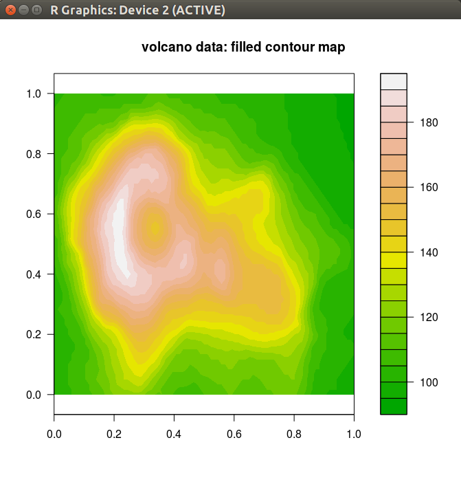

A3.1 Plot remotely - display locally

> library(future)
> plan(cluster, workers = "remote.org")

## Plot remotely
> g %<-% R.devices::capturePlot({
    filled.contour(volcano, color.palette = terrain.colors)
    title("volcano data: filled contour map")
 })

## Display locally
> g

Screenshot of example(volcano) plot

R (>= 3.3.0)
recordPlot() + replayPlot()
Replotted using local R plot routines
X11 and similar is not in play here!

A3.2 Profile code remotely - display locally

> plan(cluster, workers = "remote.org")
> dat <- data.frame(
+   x = rnorm(50e3),
+   y = rnorm(50e3)
+ )
## Profile remotely
> p %<-% profvis::profvis({
+   plot(x ~ y, data = dat)
+   m <- lm(x ~ y, data = dat)
+   abline(m, col = "red")
+ })

A3.2 Profile code remotely - display locally

> plan(cluster, workers = "remote.org")
> dat <- data.frame(
+   x = rnorm(50e3),
+   y = rnorm(50e3)
+ )
## Profile remotely
> p %<-% profvis::profvis({
+   plot(x ~ y, data = dat)
+   m <- lm(x ~ y, data = dat)
+   abline(m, col = "red")
+ })

## Browse locally
> p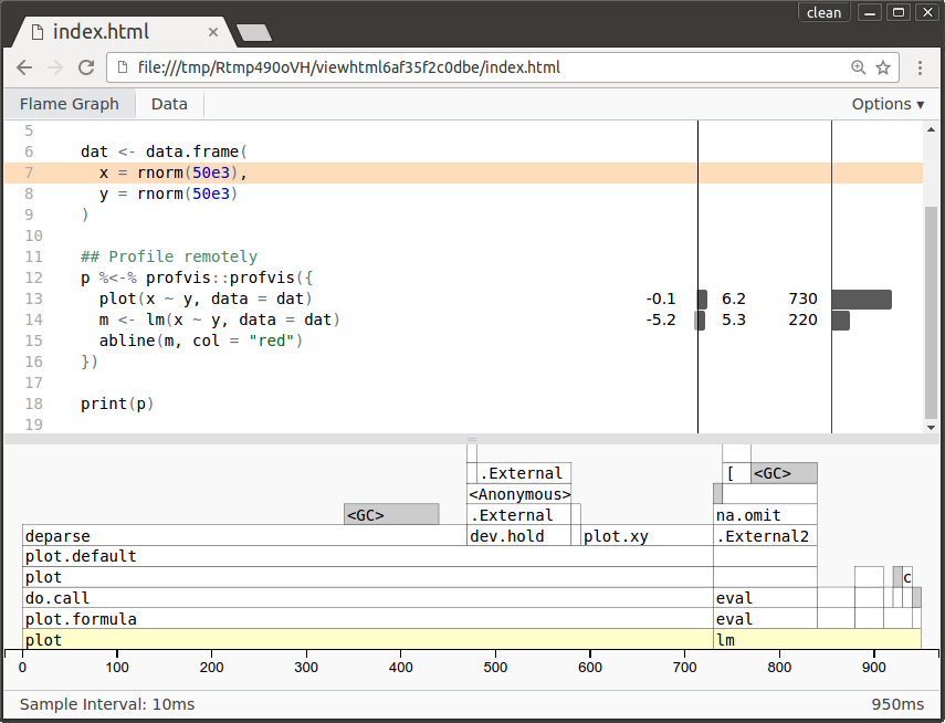

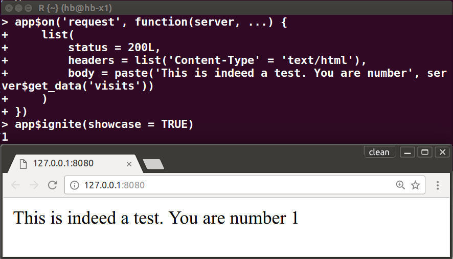
A3.2 Profile code remotely - display locally

> plan(cluster, workers = "remote.org")
> dat <- data.frame(
+   x = rnorm(50e3),
+   y = rnorm(50e3)
+ )
## Profile remotely
> p %<-% profvis::profvis({
+   plot(x ~ y, data = dat)
+   m <- lm(x ~ y, data = dat)
+   abline(m, col = "red")
+ })

## Browse locally
> p

Screenshot of profvis HTML report

A3.3 fiery - flexible lightweight web server

"... framework for building web servers in R. ... from serving static
content to full-blown dynamic web-apps"

Screenshot of fiery web server and R terminal

A3.4 "It kinda just works" (furrr = future + purrr)

plan(multisession)
mtcars %>%
  split(.$cyl) %>%
  map(~ future(lm(mpg ~ wt, data = .x))) %>% values %>%
  map(summary) %>%
  map_dbl("r.squared")
##         4         6         8 
## 0.5086326 0.4645102 0.4229655

Comment: This approach not do load balancing. I have a few ideas how support for this may be implemented in future framework, which would be beneficial here and elsewhere.

A3.5 Backend: Google Cloud Engine Cluster

library(googleComputeEngineR)
vms <- lapply(paste0("node", 1:10),
              FUN = gce_vm, template = "r-base")
cl <- as.cluster(lapply(vms, FUN = gce_ssh_setup),
               docker_image = "henrikbengtsson/r-base-future")
plan(cluster, workers = cl)

A3.5 Backend: Google Cloud Engine Cluster

library(googleComputeEngineR)
vms <- lapply(paste0("node", 1:10),
              FUN = gce_vm, template = "r-base")
cl <- as.cluster(lapply(vms, FUN = gce_ssh_setup),
               docker_image = "henrikbengtsson/r-base-future")
plan(cluster, workers = cl)

data <- future_lapply(1:100, montecarlo_pi, B = 10e3)
pi_hat <- Reduce(calculate_pi, data)
print(pi_hat)
## 3.1415

A4. Future Work

A4.1 Standard resource types(?)

For any type of futures, the develop may wish to control:

memory requirements, e.g. future(..., memory = 8e9)
local machine only, e.g. remote = FALSE
dependencies, e.g. dependencies = c("R (>= 3.5.0)", "rio"))
file-system availability, e.g. mounts = "/share/lab/files"
data locality, e.g. vars = c("gene_db", "mtcars")
containers, e.g. container = "docker://rocker/r-base"
generic resources, e.g. tokens = c("a", "b")
...?

Risk for bloating the Future API: Which need to be included? Don't want to reinvent the HPC scheduler and Spark.

↑, ←, Pg Up, k	Go to previous slide
↓, →, Pg Dn, Space, j	Go to next slide
Home	Go to first slide
End	Go to last slide
b / m / f	Toggle blackout / mirrored / fullscreen mode
c	Clone slideshow
p	Toggle presenter mode
t	Restart the presentation timer
?, h	Toggle this help